Personalized PageRank with Edge Weights

Note: This is the third article in my internal link analysis with Python series. This post will use data from the last post, “working with large link graphs,” and use techniques outlined in the first, which introduced link graph analysis with NetworkX.

PageRank can be a helpful auditing tool, but by default, it has two limitations.

1. All links have equal value. As a result, anything with a site-wide link receives a high PageRank value. It doesn’t accurately reflect link weights or diminishing returns. It’s common for Privacy Policy style pages to rank amongst the highest PageRank pages.
2. Assumes a uniform value for every page. It does not account for external links from 3rd party sites. Perhaps we want to reflect external discoverability in our score.

In this post, I’m going to customize our PageRank calculation to address those two issues. I’ll look at using link weights and Personalized PageRank.

Methods to Customize PageRank Calculations

NetworkX’s PageRank calculations have three parameters that allow us to customize our nodes and edges. They are:

1) NStart:

This assigns every node a starting PageRank value. Without this, all nodes start with a uniform value of 1/N, where N is the number of nodes in the graph. It shouldn’t change the outcome of your calculation, as PageRank should still converge on the same value as it would without. However, this can speed up the time it takes to calculate PageRank if the initial values are closer to the final value than the default uniform distribution.

2) Personalization

Personalization assigns a weight to each node that influences the random walk restart. It biases the walk towards specific nodes. Without this set, each node has a uniform probability of 1/N.

We can use this to reflect external link value. Nodes with more external links will have a greater probability of being the site’s entry point (the starting point of a random walk).

You can also use this to measure the centrality relative to a specific node or subset of nodes. We can label a subset of nodes and give them personalization values. Outside of SEO, this could be used for recommendation systems, spam detection, and fraud detection by finding which nodes are most discoverable relative to a specified subset.

3) Weights

Edge weights change the relative value that each link contributes. By default, all edges are given a uniform value of one. We can use this attribute to have NetworkX pass less value through certain edge types.

We explored link positions in the last post and used them to assign link scores, which we can use for weights. This allows us to label certain link types, such as footer links and other boilerplate links, as low-value internal links.

Weights can also account for the diminishing returns links experience as the inlink count goes up. You can reduce the weight of edges that go to a page with an extreme inlink count.

Customizing PageRank

Let’s use a simple four-node graph to demonstrate the concepts, and then I’ll use our real-world demo site. I’ll try not to explain the code covered in the previous posts but will try to mention anything new.

Imports

We will use NetworkX to look at our link graph, Matplotlib to visualize, Pandas to manipulate our data, and NumPy for some math calculations.

import matplotlib.pyplot as plt
%matplotlib inline
plt.rcParams.update({
    'figure.figsize': (9, 9),
    'axes.spines.right': False,
    'axes.spines.left': False,
    'axes.spines.top': False,
    'axes.spines.bottom': False})
import networkx as nx
import pandas as pd
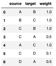
import numpy as np

Import Data Set

inlinks_csv = 'data/pagerank/pr-demo.csv'
df = pd.read_csv(inlinks_csv)
df

Output:

Read into NetworkX Graph

I’m going to import the same edgelist twice as two separate graphs. The first won’t have weights, but the second one will. We can compare the differences in PageRank when edge weights are included.

Unweighted Graph:

G=nx.from_pandas_edgelist(df, 'source', 'target', create_using=nx.DiGraph)

Weighted Graph:

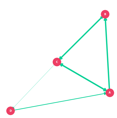
G_weighted=nx.from_pandas_edgelist(df, 'source', 'target', create_using=nx.DiGraph, edge_attr='weight')

Visualize Unweighted Graph

Let’s visualize the graph quickly, so we can see what we’re working with. The one bit of new code scales up the weight values to a practical edge width value.

weights = [i * 5 for i in df['weight'].tolist()]

pos = nx.spring_layout(G, k=0.9)
nx.draw_networkx_edges(G, pos, edge_color='#06D6A0', arrowsize=22, width=weights)
nx.draw_networkx_nodes(G, pos,node_color='#EF476F', node_size=1000)
nx.draw_networkx_labels(G, pos, font_size=10, font_weight='bold', font_color='white')
plt.gca().margins(0.1, 0.1)
plt.show()

Here is our graph.

Calculate Personalized & Weighted PageRank

I’m going to calculate PageRank five different times. Each calculation uses a slightly different combination of parameters. This will help us see what each approach does.

Variants of PageRank

• Simple PageRank: This is the default PageRank with no customization. It is the score you’ll get from most tools and tutorials. All links and nodes have equal value.
• Personalized PageRank:  Uses the personalization parameter with a dictionary of key-value pairs for each node. I set node C to a value of 1 and all other nodes to zero. When the random walk restarts, it will bias C. Perhaps C is the only node with external backlinks.
• NStart PageRank: This sets an initial PageRank value for each node. It’s done with the nstart parameter using the same dictionary approach. I set node C to a PageRank of 1 (highest possible PageRank) and all other nodes to zero. Initial PageRank is usually a uniform 1/N.
• Weighted PageRank: This uses the second graph I imported, which includes edge weights. This will devalue some edges based on their weight.
• Weighted Personalized PageRank: This combines the two approaches. It uses the graph with edge weights and applies the same personalization dictionary as before.

I’ll store these all in a DataFrame.

simple_pagerank = nx.pagerank(G, alpha=0.85)
personalized_pagerank = nx.pagerank(G, alpha=0.85, personalization={'A': 0, 'B': 0, 'C': 1, 'D': 0})
nstart_pagerank = nx.pagerank(G, alpha=0.85, nstart={'A': 0, 'B': 0, 'C': 1, 'D': 0})
weighted_pagerank = nx.pagerank(G_weighted, alpha=0.85)
weighted_personalized_pagerank = nx.pagerank(G_weighted, alpha=0.85, personalization={'A': 0, 'B': 0, 'C': 1, 'D': 0})

df_metrics = pd.DataFrame(dict(
    simple_pagerank = simple_pagerank,
    personalized_pagerank = personalized_pagerank,
    nstart_pagerank = nstart_pagerank,
    weighted_pagerank = weighted_pagerank,
    weighted_personalized_pagerank = weighted_personalized_pagerank,
))
df_metrics.index.name='urls'
df_metrics

The Effect of PageRank Parameters

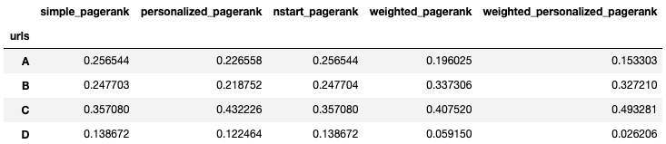
Simple PageRank is our reference PageRank for comparison. C had the highest score and D is the lowest, with A and B being nearly equal. Even though the one link to D is a weak link, it still has a decent PageRank score.

Let’s move across to the right and compare each method.

Comparing Scores

• Personalized: Node C, set to 1, went up, and all other nodes went down. The relative distribution of the other three nodes is similar, but all went down a bit. Node D still has a decent PageRank.
• NStart: It’s the same as Simple PageRank. Even though C has a value of 1 to start, and all other nodes have zero, the iterations of PageRank still converged on the same value.
• Weighted: The distribution of PageRank has shifted. D has lost a considerable amount of PageRank, and A has lost a little bit of PageRank. B and C have the greatest number of full-value links, so they went up the most.
• Weighted Personalized: This combines the effect of personalization and edge weights. D has reduced even further and is now very unimportant, and C now has a PageRank of 0.49 (nearly half the the total PageRank).

These adjustments can give us a dramatically different distribution than the default PageRank by allowing us to factor in additional data about the link graph.

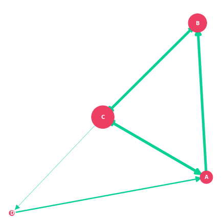
Changing Node Size with PageRank

We can now visualize our graph again and use our Weighted Personalized PageRank as the node size. This will give us a better visualization of our graph.

Set Node Size Using PageRank

I’m using the same approach I used for edge weights in the previous visualization. I’m multiplying by quite a lot to get the PR values high enough to work as node sizes.

node_size = [i * 4000 for i in df_metrics['weighted_personalized_pagerank'].to_list()]
node_size

Redraw Graph with PageRank as Node Size

weights = [i * 5 for i in df['weight'].tolist()]
nx.draw_networkx_edges(G_weighted, pos, edge_color='#06D6A0', arrowsize=22, width=weights)
nx.draw_networkx_nodes(G_weighted, pos,node_color='#EF476F', node_size=node_size)
nx.draw_networkx_labels(G_weighted, pos, font_size=10, font_weight='bold', font_color='white')
plt.gca().margins(0.1, 0.1)
plt.show()

Output:

Using a Real World Data Set

Let’s do it again with a real website.

Importing Data

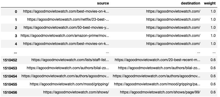
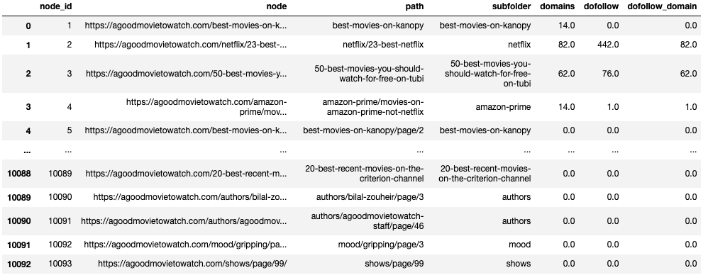
We’re going to use the edgelist and nodes from the last post in this series, which is a medium sized movie website. I’ll load them into a Pandas DataFrame and drop some columns we don’t need.

df_edgelist = pd.read_csv('data/large-graphs/edgelist.csv')
df_nodelist = pd.read_csv('data/large-graphs/nodes.csv')
df_edgelist = df_edgelist.drop(columns=['type','status_code','follow','link_position'])
df_edgelist.rename(columns={'link_score':'weight'}, inplace=True)

Our edgelist looks like this:

Data Wrangling to Fix Edge Weights

Next, I need to fix a couple of edges I missed in the last post. My link positions didn’t adequately devalue the edges for three pages that get site-wide links. Instead of recrawling, I’m going to devalue all edges with these URLs as a destination.

df_edgelist.loc[df_edgelist.destination == "https://agoodmovietowatch.com/login/", ['weight']] = 0.1
df_edgelist.loc[df_edgelist.destination == "https://agoodmovietowatch.com/unlock/", ['weight']] = 0.1
df_edgelist.loc[df_edgelist.destination == "https://agoodmovietowatch.com/why-a-premium-newsletter/", ['weight']] = 0.1

Import External Link Data

I’m going to use Ahrefs data to calculate our personalization. There are several metrics we can use, but I’m going to estimate followed domains. I used the lowest value of linking domains or “dofollow” links.

There is no need to normalize these as the PageRank algorithm already does this. It will convert each personalization value to a percentage of the sum for all nodes (this is imperfect because our Ahref data aren’t unique counts per URL, but it works well enough to get a general idea).

As always, feel free to use a different data provider and approach. Be careful with tool-provided metrics, as most of them are logarithmic. Also, be careful with raw link counts; site-wide links can inflate them (and you’ll overvalue a node).

Let’s read them into Pandas.

df_link_data = pd.read_csv('data/large-graphs/external-links.csv')
df_link_data

Join Node List and External Link Data

Next, we need to join our node list with our link data. This is the same as a VLookup in Excel. I use the node (URL) to find the corresponding data for it in both DataFrames, then merge them into a single DataFrame.

I’m using pd.merge for this. The parameters are relatively straight-forward. The “on” parameter is the column name in both DataFrames that will be used to match. It’s a unique identifier. The “how” parameter denotes the style of merging. With a left join, I will keep the elements that exist in the first DataFrame. I won’t bring in nodes that are in DataFrame 2 that aren’t in DataFrame 1. It is similar to a SQL left outer join.

link_join = pd.merge(df_nodelist,  
                      df_link_data,  
                      on ='node',  
                      how ='left') 
link_join 

Replace Empty Cells with Zero

Not all nodes in my crawl have link data. They end up with NA/NaN values after the merge. I want to replace them with zeros using “fillna.”

link_join = link_join.fillna({'domains':0, 'dofollow':0, 'dofollow_domain':0, 'url_rating':0, 'raw_url_score':0})

Our merged DataFrame looks like this. It has the original data from the node list, but the external link data has been appended.

Create Personalization Dictionary

Let’s use our new merged DataFrame to create our personalization dictionary.

personalized = pd.Series(link_join.dofollow_domain.values,index=link_join.node).to_dict()

Calculate Personalized PageRank

Let’s import our edgelist from our Panda’s DataFrame into NetworkX. I’m going to do this twice, once with edges and once without. This will let us compare the effect of edge weights.

G=nx.from_pandas_edgelist(df_edgelist, 'source', 'destination', create_using=nx.DiGraph)
G_weighted=nx.from_pandas_edgelist(df_edgelist, 'source', 'destination', create_using=nx.DiGraph, edge_attr='weight')

Calculating Multiple PageRank Variants

We’re using the same approach as before, but instead of manually entering the dictionary, we’re going to use the personalization dictionary we created a moment ago.

simple_pagerank = nx.pagerank(G, alpha=0.85)
weighted_pagerank = nx.pagerank(G_weighted, alpha=0.85)
weighted_personalized_pagerank = nx.pagerank(G_weighted, alpha=0.85, personalization=personalized)

df_metrics = pd.DataFrame(dict(
    simple_pagerank = simple_pagerank,
    weighted_pagerank = weighted_pagerank,
    weighted_personalized_pagerank = weighted_personalized_pagerank,
))

df_metrics.index.name='urls'
df_metrics

We now have a DataFrame with the three variants of PageRank. Let’s explore what changed.

How Edge Weights Changed PageRank

I’m going to insert two new columns to show how weights changed PageRank. The first contains the difference between Simple and Weighted PageRank. The second converts that difference into a percent difference.

df_metrics['weighted_difference'] = df_metrics['weighted_pagerank'] - df_metrics['simple_pagerank']
df_metrics['weighted_percent_change'] = (df_metrics['weighted_difference'] / df_metrics['simple_pagerank']) * 100
df_metrics

Problems with Default PageRank

Let’s first look at the URLs with the most and least PageRank without weights and personalization. I’ll sort by simple_pagerank. The DataFrame displayed shows the top 5 and bottom 5 rows.

df_metrics.sort_values(['simple_pagerank'], ascending=0)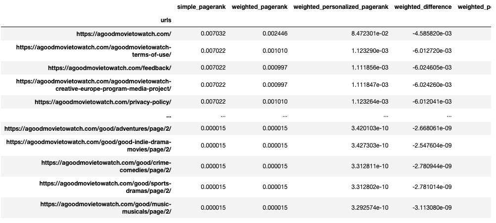

Pages like “Privacy Policy,” “Feedback,” and “Terms of Use” rank amongst the most popular pages on the site due to their site-wide footer links. This makes default PageRank less helpful. I highly doubt Google considers those the most important pages on the site.

This also tells me nothing about where the external link equity resides. Several of the pages with the greatest backlinks don’t rank in the top 5.

How Weights Improve PageRank

Let’s see how adding edge weights improved things. We can sort by the difference between simple PageRank and Weighted PageRank to find the biggest winners and losers.

df_metrics.sort_values(['weighted_difference'], ascending=0)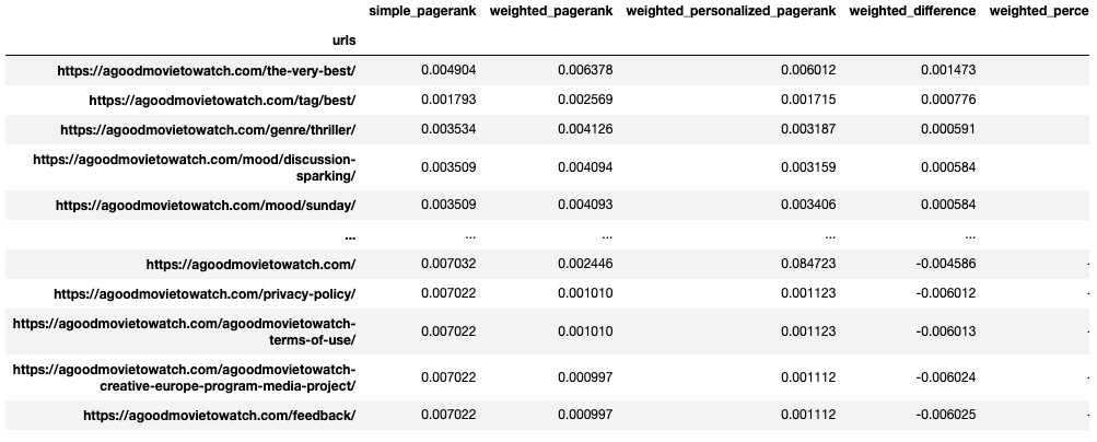

Notice how the low-value URLs with site-wide footer links had the most significant reduction in PageRank. We’ve significantly deprioritized URLs with lower-value boilerplate links. You may also notice that the homepage reduced in value because we reduced the site-wide logo link’s weight to account for diminishing returns. However, it’s still has a relatively high score, and it’ll regain PageRank from the personalization parameter (it’s the most linked URL from external sources).

The URLs with the greatest increase received more unique links from detail pages instead of relying on site-wide footer and header links.

Lastly, note that blog posts or editorial articles do not rank amongst the highest PageRank pages. They are not well-linked internally; therefore, they don’t score as high. However, they are amongst the most externally linked URLs. Let’s look at how personalization fixes this.

Backlink Adjusted PageRank

Let’s sort by Weighted Personalized PageRank.

df_metrics.sort_values(['weighted_personalized_pagerank'], ascending=0)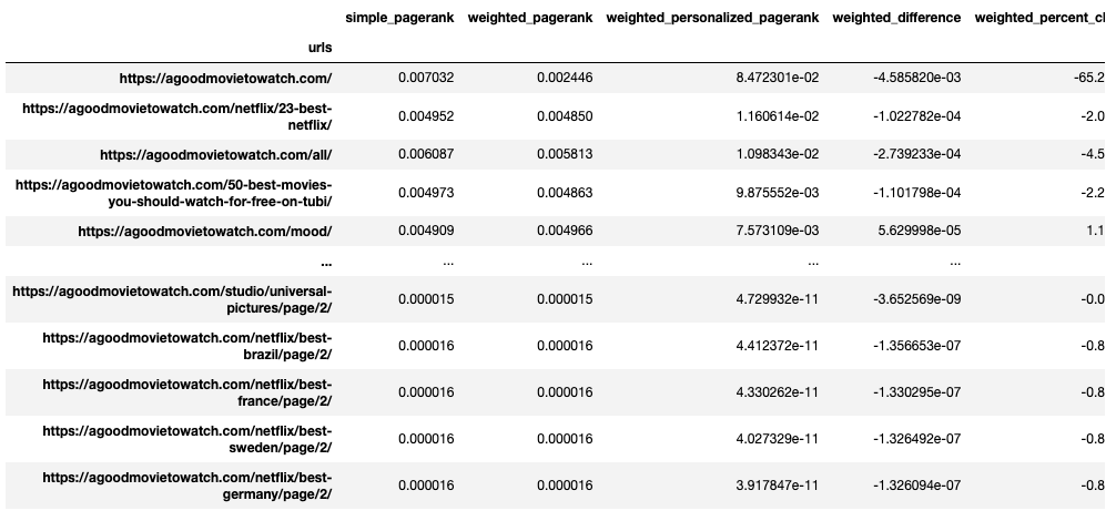

We get all of the benefits of edge weight as well as backlink data. Now several editorial articles rank amongst the most popular pages because of their backlinks. This is helpful because these URLs acquire the external link “equity” from backlinks and distribute it through internal links.

This brief look doesn’t show the full picture. Let’s visualize the PageRank as a probability distribution.

PageRank Log Transformation

Let’s convert our Weighted Personalized PageRank to a 10-point scale using a log transformation, which I talked about in-depth in my last post. This will help us interpret our results.

df_metrics['internal_pagerank_score'] = np.clip(np.round(np.log10(df_metrics['weighted_personalized_pagerank']) +10, decimals=2), 0, 10)

Note: I’m still using a constant of 10 to shift the log curve, but with the weights and personalization, the raw PageRank scores are getting relatively small. There is a risk that our transformation returns a negative value. For larger sites, you may not be able to use the constant of 10 and may need to anchor your max score to 10 (it all depends on what values you get). I explain this in detail in my last post.

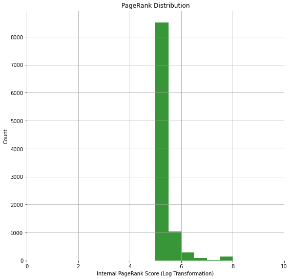
Visualize Personalized PageRank Distribution

Next we’ll plot a histogram and compare it to the default (simple) PageRank distribution.

bins = [0.5, 1, 1.5, 2, 2.5, 3, 3.5, 4, 4.5, 5, 5.5, 6, 6.5, 7, 7.5, 8, 8.5, 9, 9.5]
n, bins, patches = plt.hist(list(df_metrics['internal_pagerank_score']), bins, facecolor='g', alpha=0.75)
plt.xlabel('Internal PageRank Score (Log Transformation)')
plt.ylabel('Count')
plt.title('PageRank Distribution')
plt.xlim(0, 10)
#plt.yscale('log')
plt.grid(True)
plt.show()

Simple PageRank:

Weighted Personalized PageRank:

I believe the new distribution is a more accurate representation of link value distribution on the website.

The reduction in boilerplate link edges helped demote the small number of pages with runaway PageRank due to site-wide links. This helped even out our distribution.

Our PageRank now looks more like a normal distribution, with the bulk of the distribution falling in the middle. After manually reviewing the site, this seems fair. They do a lot of in-content cross-linking. Their detail pages have a lot of attribute links like genre, mood, actors, and directors. Most of their category pages have side-bars that cross-link between their categories. This helps pull more pages into the center.

Also, note that our range has increased. With Simple PageRank, our scores were between 5 and 8, but with weights and personalization, they range from 0 to 8.5. This gives us more fidelity. We don’t have everything crammed into a small range between 5 and 5.5. The default PageRank calculation assigns no pages a very low score, but now our pagination pages have a value less than 1.

Lastly, we have more insight into what needs more or less PageRank to improve performance. It changes our internal linking prioritization. Perhaps we don’t need to improve the visibility of a URL with low internal inlinks because it has external link value (and is less dependent on internal links). We now capture both concepts in a single metric.

Export PageRank to CSV

We can easily export our metrics to CSV for analysis in Excel. Before exporting, I’m going to drop all the variants and comparison columns. I may just want the Weighted Personalized PageRank. Perhaps you want to keep them all so you can compare the effect of link types and external links.

df_metrics = df_metrics.drop(columns=['simple_pagerank','weighted_pagerank','weighted_percent_change', 'weighted_difference', 'weighted_percent_change'])
df_metrics.to_csv('data/large-graphs/custom-pagerank.csv')
df_metrics