Working With Large Internal Link Graphs in Python

Note: This is the second post in my series on analyzing internal link graphs with Python. If you haven’t read the first post, I recommend reviewing it before continuing. I’m picking up where I left off. While the goal of this post is ultimately graph analysis, the techniques in this post work for data wrangling large CSVs in general.

In the last post, I covered the basics of NetworkX, a great, easy-to-use Python package for analyzing network graphs. I used a tiny network to demonstrate concepts, but the link graphs SEOs work with are much larger and come with unique challenges. In this post, we’ll explore some techniques for managing large data sets.

This post will focus on data wrangling, memory management, and graph reduction as a method for managing large graphs. If those techniques aren’t enough, I’ll share some C/C++ libraries (that work with Python) that are much faster than NetworkX.

This is quite a long post, so here is a table of contents for those who want to quickly jump around or skip the introductory material.

Table of Contents

• Large Data Set Challenges
• Working with Large CSVs in Pandas
• Pandas Basics
  • Reducing Panda Memory Usage
• Data Wrangling
  • Discovering & Profiling
  • Structuring & Extracting
  • Cleaning Our Data
    • Multigraph for Parallel Edges
    • Calculating Link Scores
    • Deduplicating Edges
    • Canonicalization
  • Enriching our Dataset
    • Classifying URLs
    • Parsing Node URLs
    • Assigning Node IDs
• Exporting DataFrames to CSV
• Read NetworkX Graph from Pandas
• Can NetworkX Handle Larger Graphs?
• Describing Our Graph
  • Weakly Connected Graphs
  • Exporting Our Centrality Scores
• Analyzing Our Centrality Metrics
  • Scaling Our Metrics
  • Understanding PageRank
  • Visualizing a Probability Distribution
  • Log Transformation & 10-point PageRank Scale
• Resources for Graphs with More Than 100K Nodes
• Comparing Graphing Packages
• Introduction to iGraph

Large Data Set Challenges

We run into a variety of problems when dealing with large CSVs, but some of the common ones are:

• Too large to open in Excel: Excel allows a maximum of 1,048,576 rows, so it can’t help us with CSVs with millions of rows.
• Hard to see it all: When you have 100 million rows of data, it’s challenging to look at it all, to know what you have, or what you’re missing.
• Messy, hard to clean, and data gaps: Imperfections occur in large data sets. They can require extensive cleanup work. Perhaps we need to append or extract data. The difficulty of this can scale with size.
• Extraneous data: Exports may include more data than we need for analysis, such as extra columns or rows. These need to be trimmed before analysis can begin.
• Too large for our memory: At some point, even with tools in Python, data can be too large for our machines to manage. There are techniques available to use the memory and CPU we have more efficiently. The answer may mean a faster machine, but let’s try to maximize what we can do with what we have.
• Hard-to-understand metrics and analysis: Statistics and calculations on large datasets can have increased complexity. The outputs may also be hard to understand. For example, PageRank calculations on large graphs typically output tiny numbers with a heavy-tailed and skewed distribution. These metrics can be less intuitive to interpret.

I’ll go through a handful of techniques that can help us address these common problems. 

How Large is Large?

SEOs work on a diverse set of clients, so “large” is relative. I want to be as inclusive as possible. For many small-to-medium sites, this data wrangling can be done in Excel. For this post’s purpose, I’ll consider anything larger than 1 million rows large enough to create problems.

They can get large enough to require a different solution than the ones I’m covering today. However, this post should help the majority of SEOs for the majority of their client work.

For NetworkX, a graph with more than 100K nodes may be too large. I’ll demonstrate that it can handle a network with 187K nodes in this post, but the centrality calculations were prolonged. Luckily, there are some other packages available to help us with even larger graphs.

For today’s demo, I will use two larger graphs that I feel are representative of sites many SEOs will work with. I”ll use the first one for the majority of the post, but I’ll quickly show that the larger one also works.

Site 1:

• Non-client movie content website
• 1.44 GB Screaming Frog inlink export
• 4,437,284 rows x 14 columns
• I have no affiliation with this site. I just needed data for demonstration purposes, and I like watching good movies.

Site 2:

• E-commerce site
• 14.74 GB Botify inlink export
• 98,293,232 rows x 7 columns

Your Computer as a Bottleneck

Large can be defined by the machine you’re using. Your biggest bottleneck is likely your ram. You can increase the graph sizes you can handle by upgrading the machine you’re using. That may not be the cheapest or easiest way to scale your analysis, though.

Some algorithms take advantage of multiple threads, but some don’t. There are also other solutions like chunking your imports or using parallel computing libraries. I won’t cover those today but will provide some resources at the end of this post. 

I’m using an M1 Mac Mini with 16 GB of ram to demo this analysis. I wanted to show that you don’t need a costly machine to handle the most common use cases an SEO will encounter.

Your Problem May Be Your Data

If you’re running into issues with NetworkX on a medium to a large network, evaluate the data you’re ingesting. You may find that you’re loading more into ram than you need to.

Here are a few common issues found in inlink exports:

• Links to static assets and images
• Nodes for page types you don’t need to consider
• Non-canonical nodes
• Nodes with only one inlink
• Links to 3XX, 4XX, and 5XX URLs
• 301 redirects, canonicals, and 301/canonical chains
• Robots Disallowed URLs
• Nofollow links edges
• Noindexed URLs
• Thin, duplicate, parameterized URLs
• Large labels (full URL) instead of node ID or path only labels
• Loading the full site when a few sections will do
• Not consolidating nodes
• Not canonicalizing URLs

What you load into your graph depends on your goal. Perhaps you need to load everything, but we can often find the tactical insights we need with a much smaller representative data set.

Working with Large Export CSVs

If your inlink export has less than a million rows, you can do your data cleanup in Excel. For larger CSVs, we can use the Pandas package in Python. There is a bit of a learning curve, but it’s intuitive once you get used to it.

(If you’re using Excel, be sure to delete blank rows and unused columns before reading into NetworkX. These can sometimes be saved to your CSV and cause problems. You can also open the CSV in a text editor and manually delete them.)

What is Pandas?

Pandas is a Python package with tools for data manipulation and analysis. Essentially, it’s a programmatic Excel.

I recommend checking out Panda’s 10 Minute starter guide. They have a lot of excellent documentation and a cookbook with “recipes” for common problems. There is a great community as well. You can find most of your problems answered on Stack Overflow or YouTube.

Jupyter Notebooks

Jupyter Notebooks is a helpful tool for data analysis and data wrangling. If you’re not familiar with Jupyter Notebooks, think of it as a Google Doc that lets you have code cells that run Python inline. You can display results inline, view charts, and annotate with notes along the way. You can also use Google Colab, which is a hosted version of Jupyter Notebooks.

I recommend using Jupyter Notebooks for the type of data wrangling we’ll cover in today’s post.

It’s easy to install and use.

Install it with pip in terminal:

pip install notebook

Run it in terminal:

jupyter notebook

It’ll open in your browser using localhost. You can find the documentation here, but there are also many great videos on YouTube. Because I’m using a notebook, I don’t have to use “print()” to see my results.

(You can install all the packages I mention today using the same pip method. If I import a package you don’t have installed, be sure to install it first.)

Pandas Basics

Before we look at a real dataset, let’s cover some of the basics.

First, you’ll need to install Pandas by typing “pip install pandas” into your terminal (pip3 for Python 3 on Mac). We’ll also need to import Pandas to use the package.

import pandas as pd

Panda’s Data Structures

Panda has two primary data structures that we’ll be using.

• Series: A one-dimensional labeled array. Think of these as one column of a spreadsheet with index labels. When we select one column from a data frame, we get back a Series.
• DataFrames: A two-dimensional labeled data structure. Think of it like a spreadsheet or SQL table with rows and columns.

Reading CSV Data into a DataFrame

For this introduction, I’ll use our scenario one dataset from the last post, and then I’ll switch over to our more extensive data set.

Pandas has functions to read data from several different formats. We can use “read_csv” to import our inlink CSV data. You could also use read_excel for Excel files. If your CSV has more columns than we need to import, we can define the subset of columns we want to import. Use the names of the columns (first-row value) in your CSV.

columns = ['Source', 'Target']
df = pd.read_csv('data/scenarios/s1.csv')[columns]

We now have the CSV loaded into the DataFrame “df.”

Check Size (Shape) of DataFrame

Let’s check how many rows and columns we imported.

df.shape

Output: (40, 2)

Check Columns

I can also check the names of the columns in the DataFrame.

df.columns

Output: Index([‘Source’, ‘Target’], dtype=’object’)

We can see that we have two columns with the names “Source” and “Target.”

Check First N Rows

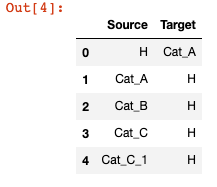
If we have a large DataFrame, we can just get the first few rows to preview our data.

df.head(5)

Output:

Look at a Range of Rows

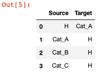
We can also select a range of rows to return.

df.iloc[0:4]

Output:

Select a Specific Cell

We can look up the value in a specific cell using its row and column numbers.

df.iloc[3, 1]

Output: ‘H’

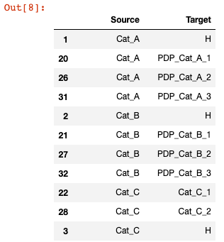
Sort Columns

df.sort_values(['Source', 'Target'], ascending=[1, 1])

Output:

Filter by Values in Columns

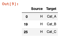
Let’s filter to rows where Target is Cat_A, Cat_B, or Cat_C.

df_cat = df.loc[(df['Target'] == 'Cat_A') | (df['Target'] == 'Cat_B') | (df['Target'] == 'Cat_C')]
df_cat

Output:

Now that we’ve covered some of the basic functionality, let’s briefly look at memory management.

Reducing Pandas Memory Usage

Reducing the memory usage of our DataFrame is helpful when working with large datasets, as it’ll allow us to work with more data and speed up our analysis in Pandas.

Datatypes

When data is loaded into a DataFrame, it uses several different data types (dtypes). They have different properties, change how values are treated in analysis, and use memory differently. Most of these are what you’d expect: Integer, Floating Point Numbers, Boolean, and Date/Time.

When there are mixed data types per column, they’re often stored as objects (also the data type used for strings). Pandas does a pretty good job of detecting the right data type, but we may want to change it for various reasons. If there are mixed data types in a column, you may get a warning, and it will use the object data type.

Categorical Data Types

Categorical data types can help you have a relatively small number of unique values relative to rows. What the categorical data type does is assign each unique value a unique id to lookup. That ID is stored instead of the string. The individual strings are stored in a lookup.

We don’t need the string until we’re ready to use it. This reduces the memory usage of our DataFrame by not requiring a string to be stored hundreds of thousands or millions of times over and over. As a result, we can load in larger data sets and work with them faster than if we left strings as objects.

This helps inlink exports because while we may have hundreds of thousands or millions of edges, we may only have 10k to 100k unique URLs. We don’t need two columns of the same 20k URLs repeated hundreds of thousands of times and wasting our memory usage.

Working with categorical data does change a few things, but I’ll highlight those as we go.

Check Our Data Types

First, let’s check which data types we’re currently using.

df.dtypes

Output:

Source object
Target object
dtype: object

Our columns are using the object data type because they are strings.

Check DataFrame Memory Usage

Next, let’s see how much memory our DataFrame is using broken down by column.

df.memory_usage(deep=True)

Output:

Index 128
Source 2566
Target 2530
dtype: int64

We’re not using much memory, but this process will be helpful once we load in a data set with more rows.

We can also sum these values to see the memory usage of the entire DataFrame. This just sums the values above.

df.memory_usage(deep=True).sum()

Convert to Categorical and Reduce Memory

I’m going to do a few things here to demonstrate the effect on memory usage.

• Make a copy of our DataFrame
• Loop through the columns I want to switch to categorical
• Set those columns as type “category”
• Calculate the ratio of the memory usage between the original and categorical copy DataFrames
• Print the results

df_small = df.copy()

for col in ['Source', 'Target']:
    df_small[col] = df_small[col].astype('category')
    
reduction = df_small.memory_usage(
    deep=True).sum() / df.memory_usage(deep=True).sum()

f'{reduction:0.2f}'

Output: 0.74

We reduced the memory usage by 26% by switching the strings to categorical. This doesn’t sound like a lot, but when we apply it to our larger data set, it will reduce memory usage by 97%.

Technically, I could have applied the “astype” to the entire DataFrame, as I’m changing the data type for all columns. However, we may have a DataFrame with more columns that we don’t want to convert. I’ll give an example of changing the entire DataFrame later.

Now that we’ve covered some of the fundamentals of Pandas, let’s start preparing our data.

Data Wrangling

Data wrangling is the process of cleaning, preparing, structuring, and enriching out data. Our goal is to take messy, unwieldy data and turn it into something useful. In doing this, we’re reducing the size of the data we have to work with.

There are roughly 6 stages of data wrangling, but these aren’t mutually exclusive. You’ll likely go back and forth between these stages.

1. Discovering & Profiling: Understand and summarize the data
2. Structuring & Extracting: Organize and optimize the data
3. Cleaning: Improve the quality of data
4. Enriching: Add additional data
5. Validating: Confirm data consistency and accuracy
6. Publishing: Publish for use and document data wrangling steps

I’m going to walk through a demonstration of this process’s first few steps using crawl data from Screaming Frog, but the work you’ll need to do may vary depending on your data source and goals for your analysis.

Getting Started

Before we start, let’s get all of our imports and data sets out of the way. I’ll explain each of these packages as we get to them. Additionally, I’m defining the location of several Screaming Frog exports upfront, so you can easily swap them with your exports. I will use them to canonicalize all the URLs in our graph and explain how to find them later in the post.

#Import Packages
import pandas as pd
import numpy as np
import matplotlib.pyplot as plt
import networkx as nx
from urllib import parse
from scipy import stats

#Display charts inline
%matplotlib inline

#Use this if you want to suppress warnings
#warnings.filterwarnings('ignore')

#Data Sets - Based on Screaming Frog Exports

#Inlink Report
inlinks_csv = 'data/large-graphs/all_inlinks.csv'

#Canonical/Redirect Chains

chains_csv = 'data/large-graphs/redirect_and_canonical_chains.csv'

#Canonicalized URLs

canonicalized_csv = 'data/large-graphs/canonicals_canonicalised.csv'

#Redirected URLs

redirect_csv = 'data/large-graphs/response_codes_redirection_(3xx).csv'

Let’s start investigating our inlink export to see what we have.

1) Discovering & Profiling

First, let’s investigate what data is included in our inlink export. I’m using a Screaming Frog export. You can find this under Bulk Exports via Bulk Exports > Links > All Inlinks.

Most crawlers have an inlink export. For example, if you use Botify, you can find the inlink report in Reports > Data Exports. It’s under your export history within the “Botify Recommended Exports” section.

Read From CSV

df = pd.read_csv(inlinks_csv)

You may get a warning at this stage due to mixed data types. We’ll get to that that in a bit, but you can ignore this warning for now. We’ll be limiting our import and converting to categorical, which will fix that.

If you want to suppress warnings in Jupyter, include this after your imports.

warnings.filterwarnings('ignore')

Check the DataFrame’s Size

df.shape

Output: 4437284, 14

Our CSV has 4.4 million rows and 14 columns of data.

Check the Columns

Let’s see what columns are included.

df.columns

Output:

Index([‘Type’, ‘Source’, ‘Destination’, ‘Size (Bytes)’, ‘Alt Text’, ‘Anchor’, ‘Status Code’, ‘Status’, ‘Follow’, ‘Target’, ‘Rel’, ‘Path Type’, ‘Link Path’, ‘Link Position’], dtype=’object’)

That’s a lot of extra data we’re not going to need to build a network graph. We’ll exclude most of those columns. Some of this data is redundant, such as Status Code and Status.

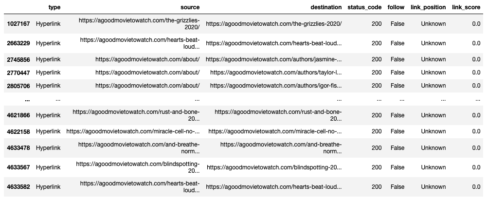
Preview First 5 Rows

df.head(5)

Output:

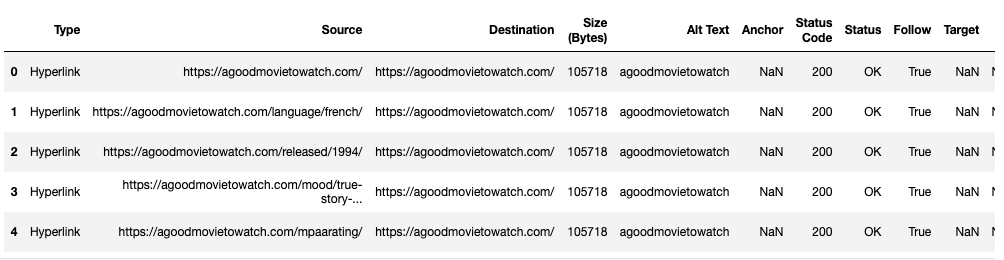
This helps us preview what kind of content is in each column. We can see the columns we don’t need, like Size, Status, and Target. What you keep depends on the goals of your analysis.

Limit our Columns

I’m going to read from the CSV again, but this time I’m going to limit the columns I bring in.

columns = ['Type','Source', 'Destination', 'Status Code', 'Follow','Link Position']
df = pd.read_csv('data/large-graphs/movie-site.csv')[columns]

Rename Columns

The column names present some challenges because of capitalization and spaces. We can rewrite these to lowercase and replace the space. This will make writing code easier. We’ll then preview our DataFrame again.

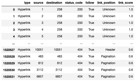
df.columns = [c.lower().replace(' ', '_') for c in df.columns]
df.head(5)

Output:

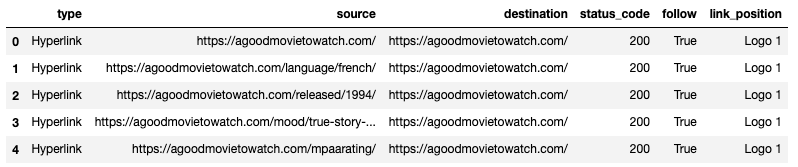
We’ve eliminated 8 columns and renamed the remaining ones to something more helpful. (If you plan to take your data back out to Gephi, it uses column names of “Source” and “Target” to identify node pairs for edges. In that case, you’ll want to name those columns appropriately.)

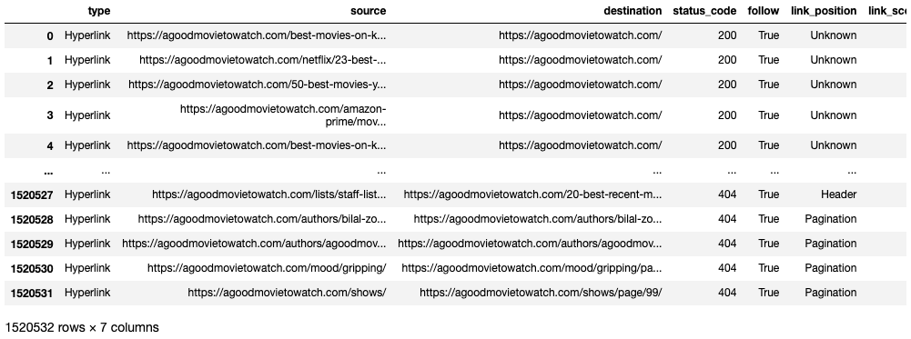
Groupby to Summarize

With 4.4 Million rows, it’s hard to know what kinds of data we have included in each column. For “source” and “destination,” it’s easy to assume they’re URLs, but what other types of values appear in “type,” “status_code,” and “link_position?”

We can use the groupby feature to “pivot” data by the values in a column (i.e., Pivot Tables in Excel). This provides a helpful summary.

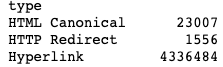
df.groupby(['type','status_code']).size()

Output:

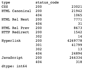
I grouped by the “type” and “status_code” columns, then used the “.size()” method to give me the count of rows with each of those values. I now know that 244K of my edges are references to JavaScript assets. I don’t need those.

Perhaps I only want to keep the links (edges) for HTML Canonical, HTTP Redirect, and Hyperlink. We’ll delete the static resources and rel=next/prev links in a moment.

This type of analysis also lets me know that my columns would work well as categorical data types. There are only 7 unique “type” values repeated in 4.4 million rows.

We can also look at our link_position data.

df.groupby(['link_position']).size()

Output:

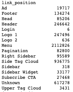
This data comes from Screaming Frog’s Custom Link Positions feature. This feature uses footprints in the HTML code to identify where on the page the link appeared. I did a quick review of the site to set a couple of link positions.

Why might we want this Link Position data?

We can set the edge’s weight based on its link position. Links that occur in the body can pass more value for those in the footer. Our centrality calculations can take this into account using edge weights.

We’ll do the data preparation in this post, but I’ll be using this data in the next post.

2) Structuring & Extracting

Next, let’s start organizing our data and make it more manageable. Let’s start by reducing its memory usage.

Convert to Categorical

Our DataFrame is using 1.44 GB of memory. This isn’t too large to be unmanageable for most computers, but let’s go ahead and reduce it anyways. We may need this for the 10GB to 30GB exports.

df = df.astype('category')

Because all of the data I have works well as categorical, I set all columns to a category data type. Again, categorical works well when there are a few unique values relative to rows.

Doing this reduces the DataFrame’s memory usage by 97%.

Removing Unwanted Rows

Now that we’ve converted our DataFrame to something more manageable let’s reduce it further by eliminating the unwanted edges (JavaScript, CSS, rel=next/prev).

drop_try_index = list(df[(df['type'] == 'CSS') | (df['type'] == 'JavaScript') | (df['type'] == 'HTML Rel Next') | (df['type'] == 'HTML Rel Prev') ].index)
df.drop(drop_try_index, inplace=True)
categories_drop = ['CSS', 'JavaScript', 'HTML Rel Next', 'HTML Rel Prev']
df.type = df.type.cat.remove_categories(categories_drop)
df.groupby(['type']).size()

I’m doing a few things here.

• Building a list of index values that I want to drop based on the “type” column’s value.
• Using that list of index values to drop rows.
• Building a list of categories that I’m no longer using (those associated with the dropped rows). Categories are kept in a different index and persist even when you don’t use them.
• Using the list of dropped categories and removing them from categories.
• Using groupby to summarize what I have left.

Output:

We’ve now excluded all the unwanted edge types.

3) Cleaning Our Data

There are many potential tasks associated with cleaning up our data that don’t apply to this data set. Our data exports from Scream Frog are pretty clean, but you can run into various issues.

For example:

• Odd formatting that requires row skips or transposing data.
• CSVs with missing or empty cells
• Cells with line breaks
• Data with non-alphanumerical data
• Cells with leading or trailing spaces (or cells with double spaces)
• Custom extractions with extraneous content or code (XPath or RegEx extractions couldn’t correctly select your data).

I won’t be covering all of these in this post, but Pandas can help with this work. You can loop through the rows of a column and perform any manipulation you wish. 

For this data set, we’ve already done some cleanup work. We’ve fixed the column names, and we’ve dropped some rows for links we don’t want. We’re going to do two more cleanup tasks for this data set.

Additional Cleaning Tasks

• Deduplicate edges when there is more than one link between Node A and Node B (and keep the most valuable link).
• Canonicalize our nodes. If a URL redirects, is canonicalized, or goes through a redirect/canonical chain, we will replace that node (URL) with its final canonical URL.

You may not want to do these two cleanup tasks depending on your goal. You may wish to keep parallel edges and non-canonical URLs for your analysis.

MultiDiGraph for Parallel Edges

NetworkX has a graph type for dealing with more than one edge between nodes in a Directed Graph. It’s called a “MultiDiGraph.” With this graph type, each edge can hold independent edge attributes. You can use this if you don’t want to consolidate edges.

There may be some analysis you can’t do with this graph type, and it will increase your edge count (and memory usage). Typically, parallel edges can be combined into a single weighted edge, but this graph type is available when you cannot.

In our example today, I won’t be “consolidating.” Instead, we’ll keep the “highest value” edge between two nodes. Alternatively, you could choose to sum the link values (and clip them to limit max value).

We don’t know precisely how Google treats parallel edges, so use your best judgment that aligns with your perspective on link scoring. If you asked 100 SEOs, you’d get 100 different answers to this. However, there is a balance between complexity and “good enough” to do the job. There is also no way to know you’re using the “right” logic.

There is the concept of the “First Link Counts” rule, but Google has shared some thoughts about it. In short, maybe, it depends, and it can change over time.

Creating a Link Position Score

To determine which edge from a set of duplicate edges to keep, we need a system for comparing their relative value. I’m going to keep one edge with the highest value edge score and delete the rest. I will start by assigning a value to a link (edge) based on its link position.

There are two reasons I want to do this:

• Only Count One Unique Edge: Node A can link to Node B multiple times from different parts of the page. This creates two edges between Node A to Node B. I want to remove these parallel edges
• Assign a Relative Value to The Link: Links can pass different values based on where the link appears. They can also count differently if they’re unique to a page versus as boilerplate link with diminishing returns We’ll convert positions into edge weights.

Assigning a Link Score

Let’s go ahead assign a link score based on the link’s position. Again, this link position came from the Screaming Frog export. Not every crawler has this feature.

score_lookup = {
    'Ad': 0.1,
    'Footer' : 0.1,
    'Header' : 0.6,
    'Logo 1' : 0.1,
    'Logo 2' : 0.1,
    'Menu' : 0.7,
    'Pagination' : 0.6,
    'Right Sidebar' : 0.9,
    'Side Tag Cloud' : 0.8,
    'Sidebar' : 0.8,
    'Sidebar Widget' : 0.8,
    'Subscribe CTA' : 0.1,
    'Unknown' : 1,
    'Upper Tag Cloud' : 0.9
}

def link_score (row):
    if row['follow'] == True :
        if row['type'] == 'HTML Canonical' :
            return 0.8
        if row['type'] == 'HTTP Redirect':
            return 0.9*score_lookup.get(row['link_position'], 1)
        if row['type'] == 'Hyperlink':
            return score_lookup.get(row['link_position'], 1)            
    else:
        return 0

df['link_score'] = df.apply (lambda row: link_score(row), axis=1)

The first thing I did was create a dictionary with key-value pairs that map link positions to a link score. I like this method more than a series of if statements.

Next, I created the function link_score() to return a score based on a few conditions. First, it checks if an edge is a “Follow” link. If a link is nofollow, it returns a link score of zero. I then check for a link type. If it’s canonicalized or redirects, I reduce the score. If it’s a Hyperlink, I look up the link position as a key in the score_lookup dictionary.

The .get() method returns the value for a specified key. The second parameter is an optional value parameter, which returns a default value if the key does not exist. I used this same method for HTTP Redirects, but I multiplied the output by 0.9 to discount it 10%.

The underlying assumptions I’m making about link scoring are:

• Boilerplate links pass less value and experience diminishing returns.
• Links in sidebars are boilerplate per section, so they’re discounted slightly but less than site-wide boilerplate.
• Links further down the page count less than those towards the top.
• Links in the footer count the least and are also boilerplate.
• Links that pass through redirects may lose some value, so I’m discounting those.
• Links that pass through canonicals may pass a bit less value than HTML links. Canonical tags are powerful but are optional to Google. They get discounted a bit due to the uncertainty.

My chosen values are arbitrary but have some basis in SEO theory. They may be wildly off base. However, I want to avoid giving too much importance to Privacy Policy style pages. If you don’t discount boilerplate links, you’ll find all your footer links as your highest PageRank URLs. Use your own best judgment and customize it.

The last bit of code goes through the DataFrame row by row, runs the link_score function, and then applies the scores. I store those values in a new column named “link_score.”

I set nofollow links to zero, which is an imperfect solution. Their value is debatable, even if they don’t pass PageRank. They still affect PageRank flow even if they don’t pass PageRank. I’ll talk about this more in a moment.

Validate Our Additions

Let’s check which edges have a value of zero.

df.loc[df['link_score'] == 0]

Output:

The edges shown with a zero link score all have their follow value set to “False.”

A better way to summarize to validate is to use groupby again.

df.groupby(['follow','link_score']).size()

Output:

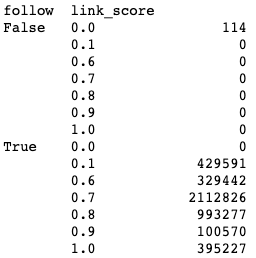
All nofollowed links (follow==False) have a link score of 0, and none of the followed links have a link score of zero.

We can also look at the link scores assigned to any give link position in our data set.

df[df['link_position'] == "Header"].groupby(['link_score']).size()

Output:

link_score
0.6 204576

All of our edges with a “Header” link_position have a link score of 0.6. We can now feel more confident that our values were assigned as intended.

Remove Nofollow Edges

Lastly, we could decide to remove our nofollow edges. This depends on your goal, but if you set their edge weight to zero, we may now want them for PageRank calculations.

Alternatively, you might want to assume that the link value flow that would have gone to a nofollow link “evaporates.” In that sense, the value of outlinks of a page is still split by the number of outbound links, even if one of those outbound links is nofollow. This prevents “link sculpting” by nofollow.

To do this, we could replace the destination of a nofollow edge with a dummy node that has no outbound links. This would create a dummy PageRank sink that collects all of the PageRank that “evaporates” due to nofollow links. I won’t do this, but we cover all the techniques needed to use this approach. Addressing nofollows with parallel edges or merged egdes may be more complicated. There is no “right” model for how to handle these.

For my dataset, only 114 edges were nofollow, and many of them may be parallel or non-canonical edges. I don’t think it’s worth the effort to account for the 114 nofollow edges in an edge list with millions of edges. It all depends on your dataset.

df = df[df['link_score'] != 0]
df.groupby(['follow','link_score']).size()

Output:

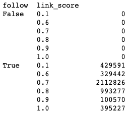
There are now no more edges with a nofollow or zero link score.

Deduplicate Link Edges

Now that we have link scores, we can deduplicate our rows and keep the edge with the greatest link score value.

df = df.sort_values(['status_code', 'link_score'], ascending=[1, 0])
df = df.drop_duplicates(subset=['source', 'destination'], keep='first')
df = df.reset_index(drop=True)

I did a few things here. First, I replaced the DataFrame with a version sorted by link score. I then deduplicated based on unique pairings of source and destination, keeping the first value (the highest link score because of the sort). I then reset the index (row ids), so they align with the number of rows I now have.

Depending on the type of analysis you’re doing, you may not want to deduplicate like this. This approach doesn’t account for anchor text differences. We might want to consolidate nodes and combine anchor text from two separate links if we’re interested in that data.

Our data frame now has 3.5 Million rows, which is down from the 4.4 Million rows of our original dataset. We have reduced our edge count by nearly 20% so far.

What if We Don’t Have Link Position Data?

You can still deduplicate or merge with all the links valued at “1” or get rid of using edge weights entirely. You can also look at other concepts like diminishing returns.

For example, the URLs with the greatest number of inlinks most likely get their links from boilerplate features like the menu or footer. You could discount the edges that point to the URLs with the greatest inlinks. This can help bake boilerplate and diminishing return concepts into your analysis.

Canonicalize Our URLs

Our export may include many duplicate and non-canonical nodes. We can canonicalize our link graph by replacing non-canonical URLs with their final destination URL (and maintain those edges).

You may not want to do this if your goal is to understand how to duplicate URLs or canonicalization issues affect your link graph. If we assume Google is decent at canonicalization, which they often are, we can go ahead and do this. This will reduce the complexity of our graph before we put it into NetworkX. Again, it depends on your goals. (I’ve also seen Google ignore canonical tags despite all of my best efforts to get them to honor it. Google will be Google.)

If you want, you could conditionally reduce the link score for edges coming from non-canonical pages, but I won’t demonstrate that in today’s post. There is no good rule of thumb on how to handle this, so adjust your link graph based on how you think about SEO theory.

Getting the Canonicalization Data

To do this, I’m going to need three supplemental exports from Screaming Frog.

• Redirect and Canonical Chains: You can find this under Reports. Look under Reports > Redirects > Redirect and Canonical Chains. This report will map out all hops between a target URL and its final destination through both 3XX redirect and rel=canonical.
• Canonicalized URLs: You can find this under the Canonicals tab. Use the dropdown to filter to “Canonicalized.” Read this guide on How to Audit Canonicals to see how.
• Redirected URLs: You can find this under the Response Codes tab by filtering to “Redirection (3XX).” I’m using this to pick up any of the 1-hop redirects that I didn’t get with the chain report.

I’m going to import each of these into their own DataFrame.

Import Chain Report

chain_columns = ['Address', 'Final Address']
chain_df = pd.read_csv(chains_csv)[chain_columns]
chain_df.columns = [c.lower().replace(' ', '_') for c in chain_df.columns]
chain_df = chain_df.drop_duplicates(subset=['address', 'final_address'], keep='last')
chain_df = chain_df.reset_index(drop=True)

I’m repeating some code we’ve gone over already. I’m reading in the CSV but limiting myself to two columns, the address and the final address. Next, I’m renaming the columns to lowercase and removing spaces. I’m then deduplicating, so I have a unique URL to destination pairs, just in case.

Import Canonicalized Report

Next, let’s import the canonicalized URL report.

canon_columns = ['Address', 'Canonical Link Element 1']
canon_df = pd.read_csv(canonicalized_csv)[canon_columns]
canon_df.rename(columns={'Address':'duplicate_url','Canonical Link Element 1':'canonical'}, inplace=True)
canon_df = canon_df.drop_duplicates(subset=['duplicate_url', 'canonical'], keep='last')
canon_df = canon_df.reset_index(drop=True)
canon_df

Import Redirects

Lastly, we can import our redirects.

redirect_columns = ['Address', 'Redirect URL']
redirect_df = pd.read_csv(redirect_csv)[redirect_columns]
redirect_df.rename(columns={'Address':'redirected_url','Redirect URL':'redirect_destination'}, inplace=True)
redirect_df = redirect_df.drop_duplicates(subset=['redirected_url', 'redirect_destination'], keep='last')
redirect_df = redirect_df.reset_index(drop=True)
redirect_df

Replace URLs with Their Canonical

Now we’re going to do the heavy lifting. We’re going to use our three new data sets, find the duplicate URL in our DataFrame, and replace it with its final URL

#Replace Canonical/Redirect Chains
df.source = df['source'].map(chain_df.set_index('address')['final_address']).combine_first(df['source'])
df.destination = df['destination'].map(chain_df.set_index('address')['final_address']).combine_first(df['destination'])

#Replace Canonical
df.source = df['source'].map(canon_df.set_index('duplicate_url')['canonical']).combine_first(df['source'])
df.destination = df['destination'].map(canon_df.set_index('duplicate_url')['canonical']).combine_first(df['destination'])

#Replace Redirect
df.source = df['source'].map(redirect_df.set_index('redirected_url')['redirect_destination']).combine_first(df['source'])
df.destination = df['destination'].map(redirect_df.set_index('redirected_url')['redirect_destination']).combine_first(df['destination'])

#Drop Duplicates and Reset Index
df = df.drop_duplicates(subset=['source', 'destination'], keep='first')
df = df.reset_index(drop=True)
df

I used the map function to substitute each value in a Series with another value. Within map, I took each of the new DataFrames and set their index (row id) to the URL we’re going to look for. I then mapped the final canonical address. The last bit, combine_first, deals with potential null values in either of the DataFrames being combined. If there is a null value in our new DataFrames, we keep the original DataFrame’s value. There shouldn’t be a null value, but just in case.

I then deduplicate again to deal with the introduction of “duplicate” canonical edges.

Output:

Remove Self-loops

Another reduction I’ll consider is removing self-loops, which is when a node links to itself. We can remove these in Pandas before creating our graph or after creating our graph in NetworkX. We can’t use some algorithms with self-loops.

Here is how we can remove them in Pandas:

df = df[df['source'] != df['destination']]

Otherwise, you can leave them and remove them in NetworkX as needed.

G.remove_edges_from(nx.selfloop_edges(G))

As you try out different functions in NetworkX, you’ll find that some of them don’t work correctly on real-world complex graphs. Some don’t work with parallel edges, some don’t work on directed graphs, and some don’t work with self-loops. It’s sometimes well-documented, but not always. If you get an error, Google it. You’ll most likely find a Stack Overflow thread explaining you can’t use the function the way you’re trying to use it.

In some cases, you can modify your data, but sometimes you can’t. Some things only work with undirected graphs or well-connected graphs. I’ll do my best to mention these as they come up.

Our Reduced DataFrame

We are now down to 1.51 million edges, which is down from our original 4.44 million edges. We reduced our edge count by 66% and generally maintained a representative link graph of our site. This is going to make it a lot easier to work with our graph in NetworkX.

There are some additional steps we could take, such as excluding the lowest value nodes, consolidating nodes, or using a subset of nodes, but hopefully, this process has demonstrated some of the concepts that can be used to reduce a large link graph. Again, how much you reduce a graph depends on your goal.

Before we jump back to NetworkX, let’s talk a bit about enriching our graph with some additional data.

4) Enriching our Dataset

As you’re working through the data wrangling process, you might want to add new data or derive data from existing data. We’ve done this a bit already by adding a link score for edge weights. However, perhaps we want to classify our nodes too.

For example, we may want to extract the unique URLs and classify them by page type or topical category. In this series’s first post, we labeled our nodes as Home, Category, or Product. We could use this data to change a node’s color or marker shape conditionally.

Visualization isn’t the only way we can use this data. We could use it filter or create a subgraph more easily.

How to Classify URLs

Getting this data can be the hard part, but here are five common ways to classify URLs easily.

1. URL Patterns: Some sites have very clearly defined URL patterns that contain data about the page type. Perhaps the URL includes a /product/ or /c/ that lets us know it’s a PDP or Category page.
2. Custom Search (Page Contains): When crawling with a tool like Screaming Frog, we can use Custom Searches to find the appearance of a word, a block of code, or CSS class/id. These can be footprints that help us identify a page’s type or topical category.
3. Custom Extraction: When crawling, we can use XPath, CSS Selectors, or Regex to extract data from the page. For example, we can extract breadcrumbs or tags to classify a page by topic.
4. Structured Data: If a page has structured data, we can extract that. It might have identifiers for the content type.
5. Analytics Tagging: Some sites used custom tagging for their analytics, which passes over additional data to their web analytics solution. This can contain valuable categorization data (as companies often use this data to slice, filter, or pivot their visit and revenue data). If there is no explicit identifier on the page or in the URL, analytics tags may be a helpful place to look.

There are also more complex methods, such as analyzing the text contents of the page. That’s out of this series’s scope, but I am working on a side project that requires this. If I’m happy with how that turns out, I’ll be sure to share it in the future.

Parsing a URL for Classification

For now, I’m going to use the site’s URL structure to give us some additional classification data. I won’t go through the full process of reviewing the data but will introduce the basic process.

If we look at a URL, we can find some helpful patterns:
https://agoodmovietowatch.com/mpaarating/r/page/1/?type=movies

From this URL, I know:

• Is a Category / Search URL
• Filters based on MPAA Ratings
• Filters to “R” rating
• Is a pagination URL (first page)
• Is filtered by parameter to movies

This URL gives me multiple bits of information I can extract to classify this URL. Let’s go ahead and categorize all URLs in our graph based on the first directory in their URL.

Create a Node List

First, let’s create a DataFrame that has all of the unique nodes in our graph. We’ll also need a node list later for iGraph.

df_nodes = pd.DataFrame(df[['source']].values.tolist() + df[['destination']].values.tolist(), columns=['node'])
df_nodes = df_nodes.drop_duplicates()
df_nodes = df_nodes.reset_index(drop=True)
df_nodes

Output:

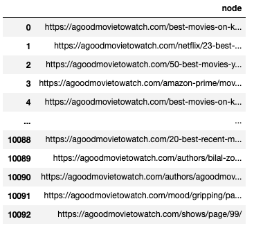
What I did is reasonably straight-forward. I selected the values in both the source and destination columns, then converted them to a list. I combined those two lists and created a new DataFrame with the column name “nodes.” I then deduplicated the list, so I’m left with unique URLs. I then reset the index. I now have a DataFrame with all the unique canonical URLs in the graph.

Parse URLs

Next, we’re going to parse the URL and extract the first directory in the path. I used urllib for this. Here is a quick demonstration of how it works.

url = "https://agoodmovietowatch.com/mpaarating/r/page/1/?type=movies"
parse.urlsplit(url).path.split('/')[1]

Output: mpaarating

I stored a URL for demonstration purposes. The final line of code is doing the work.

First, we’re going to use “parse” to split the URL. That breaks the URL into multiple sections based on the standard format of URLs. I drill in to look at the path, which would be all the stuff after the “.com”. I then use “split” to split the URL by “/,” and I want the first directory. If I used [2] instead of [1], I’d get “r.”

Next, let’s create some functions and parse all the URLs in the node DataFrame.

def node_path (row):
    return parse.urlsplit(row['node']).path.strip('/')

def node_subfolder (row):
    return parse.urlsplit(row['node']).path.split('/')[1]

df_nodes['path'] = df_nodes.apply (lambda row: node_path(row), axis=1)
df_nodes['subfolder'] = df_nodes.apply (lambda row: node_subfolder(row), axis=1)

df_nodes

Output:

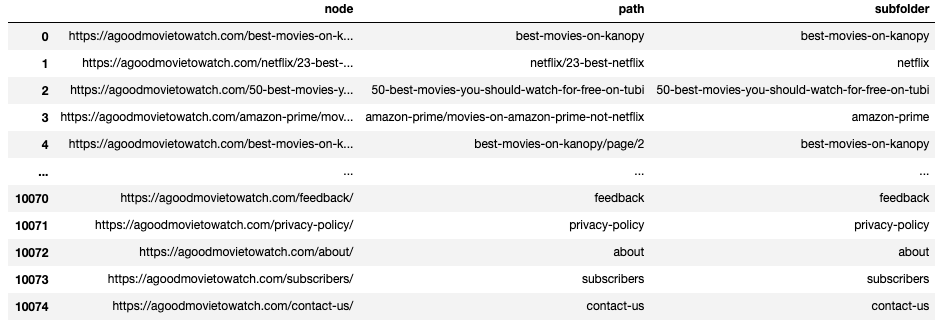
I created two functions that do nearly the same thing. One takes in a URL and returns the entire path; the other splits the path and returns the first directory. The first function uses “.strip(),” which strips the slashes off of the start and the end of the path. The second function use “split(),” which breaks the URL path up.

I created the path function because I wanted to store the path as an alternative label. If I want to show labels in a graph, this is cleaner than the full URL.

Next, the code runs through the nodes DataFrame, extracts the path and subfolder, and adds them as new columns.

We can now groupby subfolder to find our most common page types by URL directory.

Creating Node Ids

The last thing I want to do is assign every URL in the node list a unique ID. This will give me an alternative node name beside the URL. URL strings can be quite long, so I can reduce my graph’s memory size a bit by using simple ids. I don’t need to know the full URL to run calculations, and we can always add it back later by merging two DataFrames (similar to a Vlookup in Excel).

ids = range(1, len(df_nodes) + 1)
idx = 0 
df_nodes.insert(loc=idx, column='node_id', value=ids)
df_nodes

Output:

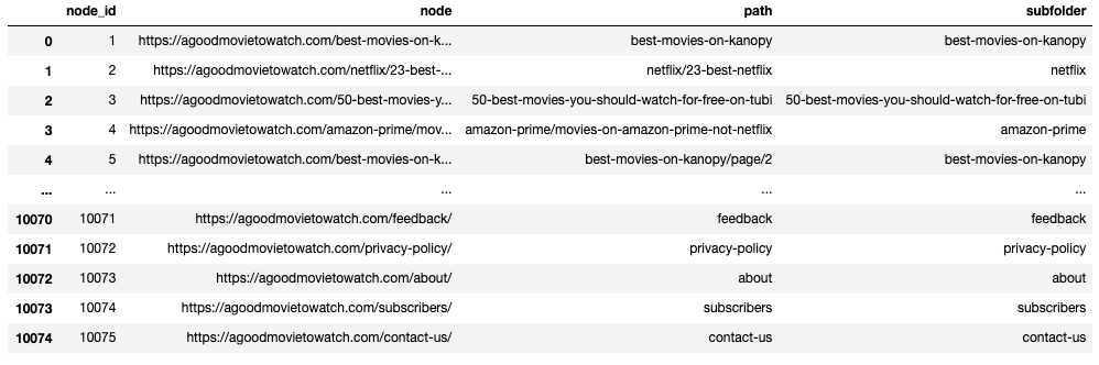
I created a list of numbers between the range of 1 and the length of the DataFrame + 1 (since it starts at zero). I then insert those values into a new column named “node_id.” The loc=idx=0 is defining where the column should be inserted. I wanted it to be the first column, so I inserted it at position 0.

Replacing URLs with ID in Edge list

Our node list provides a helpful lookup table, but we may need a new edge list DataFrame with the node ids instead of URLs. Let’s use map again to replace the URLs with their node id.

df_node_ids = df.copy()
df_node_ids.source = df_node_ids['source'].map(df_nodes.set_index('node')['node_id']).combine_first(df_node_ids['source']).astype(int)
df_node_ids.destination = df_node_ids['destination'].map(df_nodes.set_index('node')['node_id']).combine_first(df_node_ids['source']).astype(int)
df_node_ids

Output:

I created a copy of my edge list DataFrame, so I can keep the original I then used the same code from our canonicalization replacement to replace URLs with their node id.

When reading in an edgelist with NetworkX, you can change the data type for a node from a string to an integer using the nodetype parameter. There is also a function to convert node labels to integers.

We can reduce our DataFrame further by dropping columns like type, status_code, follow, and link_position. We don’t need them anymore. Our new edgelist is now much smaller than our original inlink export.

We’ll drop these columns later in the post when we use iGraph. For NetworkX, these extra columns are easy to ignore.

Export our DataFrames to CSV

Lastly, before importing our DataFrames into NetworkX, we may want to save our DataFrames to CSVs.

df.to_csv(r'data/large-graphs/edgelist.csv', index = False)
df_nodes.to_csv(r'data/large-graphs/nodes.csv', index = False)
df_node_ids.to_csv(r'data/large-graphs/edgelist_with_ids.csv', index = False)

Loading NetworkX Graph from Pandas

If you’re not familiar with NetworkX or haven’t read the first post in this series, now is an excellent time to check out my post on Internal Link Analysis with Python where I explain NetworkX and centrality metrics in detail.

We can now import our edge list into NetworkX from CSV, as we did in the last post, or import directly from our DataFame that is already loaded into memory.

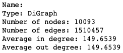
G=nx.from_pandas_edgelist(df, 'source', 'destination', create_using=nx.DiGraph)
print(nx.info(G))

Output:

Depending on your graph’s size (and the memory on your computer), you may not want to continue with the same notebook. You can start a new notebook and import the CSVs we exported earlier.

Depending on the size of your graph, it may be worth restarting your kernel and clearing out your memory. You may even want to restart your computer, avoid opening memory-intensive apps, and close any unnecessary background processes using your memory. You’ll need all the memory you can get for centrality calculations and visualization.

Can NetworkX Handle Even Larger Graphs?

Yes, but be prepared for much longer calculation times on algorithms. And even if you can run the calculations, you may not be able to visualize the entire graph at once.

I ran through a very similar process with one of my client’s inlink exports and successfully reduced the graph and loaded it into NetworkX. I can’t share this site’s details, but I wanted to demonstrate that this process can work with relatively large sites.

DataFrame Size:

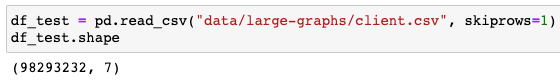
It had 98,293,232 rows of data. By converting it to a categorical data type, I reduced its size in memory by 97.1%, bringing the DataFrame down to 1.02GB.

NetworkX Graph Size:

I was able to load it into NetworkX and run centrality calculations.

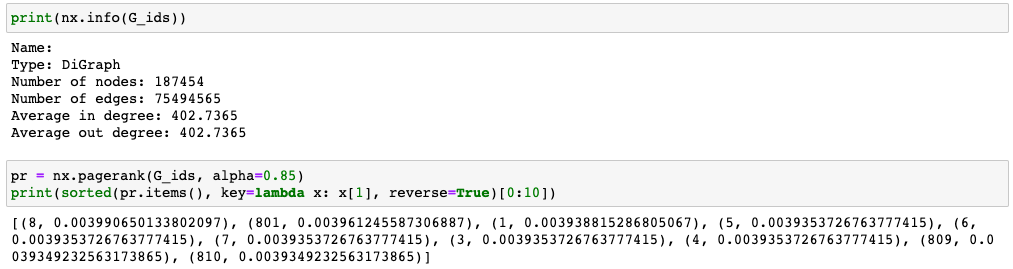
My final graph had 187,454 nodes and 75,494,565 edges. I was able to remove nearly 23M edges from the export before loading it into NetworkX.

The PageRank calculation took some time, though. I let it run in the background after work. While NetworkX was able to handle this calculation, the C/C++ libraries at the end of this post are much faster for graphs of this size.

Describing Our Graph

Note About Large Graph & Time:

If you have a larger graph, expect the next several examples to take a while. Many of the descriptive calculations and centrality metrics require a lot of computation and ram. It could take a few minutes to a few hours, depending on your graph size, what you’re calculating, and your computer. If you’re using a notebook to code, put the heavy calculations in their own cell and store the output in a variable. You don’t want an error in the subsequent code in a cell to force you to rerun the NetworkX calculation. Lastly, if you walk away from your computer, make sure it doesn’t go to sleep.

With our graph loaded in NetworkX, we can run our basic descriptive calculations.

num_nodes = nx.number_of_nodes(G)
num_edges = nx.number_of_edges(G)
density = nx.density(G)
transitivity = nx.transitivity(G)
avg_clustering = nx.average_clustering(G)
print("Number of Nodes: %s" % num_nodes)
print("Number of Edges: %s" % num_edges)
print("Density: %s" % density)
print("Transitivity: %s" % transitivity)
print("Avg. Clustering: %s" % avg_clustering)

Output:

Number of Nodes: 10093
Number of Edges: 1510457
Density: 0.01482896537429806
Transitivity: 0.813288053363458
Avg. Clustering: 0.7683919618640551

Weakly Connected Graphs or “Infinite Path Lengths”

Some calculations we discussed in the last post may not work for real-world link graphs because they are “weakly connected.” For example, Eccentricity doesn’t always work on Directed Graphs. This means other functions like Diameter, which depends on Eccentricity because Diameter is max Eccentricity, also do not work.

Eccentricity finds the path between each node and every other node on the graph. Directed Graph paths are one-way. There may be nodes with a path to them, but not a path out that finds its way back to every other node. Perhaps there are no outlinks on a node, or maybe the outlinks don’t follow a path back far enough towards the “center” of the graph to fork back off to another section. If this happens, then NetworkX can’t find a path from a node to all other nodes. When NetworkX sees this, it returns this error: “networkx.exception.NetworkXError: Graph not connected: infinite path length.” That error is returned when the number of nodes reachable from a given node does not equal the network’s total number

This error is not entirely accurate. If NetworkX ran into this problem on an Undirected Graph, it would mean that part of the graph is disconnected from the rest of the graph. For a Directed Graph, it could mean that graph is disconnected, but it’s also very likely the graph is “weakly connected.”

We typically use crawler data for our SEO analysis, which means the crawler had to see a link to discover a page. This makes it very unlikely that our export contains a disconnected graph. There is always a risk that we accidentally disconnected the graph during our cleanup efforts. There is also the risk for an unconnected graph if our crawler seeks to find orphan URLs (discovery from XML Sitemaps, GSC, analytics, logs, etc.).

Running Eccentricity on a Weakly Connected Graph

The solution for this is relatively simple. We convert the graph to an undirected graph for the subset of functions that fail to calculate an Eccentricity. This lets the network transversal go back the way it came. The output you’ll get isn’t really accurate for your graph since links aren’t bidirectional, but it’s the best we can do (or that I’ve learned so far).

Doing this is really simple:

diameter = nx.diameter(G.to_undirected())
center = nx.center(G.to_undirected())
print("Diameter: %s" % diameter)
print("Center: %s" % list(center))

We append “.to_undirected()” to our graph variable G before applying a function to it. This type of calculation can take some time. NetworkX has to transverse your graph from every node to every other node.

Output:

Diameter: 4

Center: [‘https://agoodmovietowatch.com/all/’, ‘https://agoodmovietowatch.com/’, ‘https://agoodmovietowatch.com/privacy-policy/’, ‘https://agoodmovietowatch.com/agoodmovietowatch-terms-of-use/’, ‘https://agoodmovietowatch.com/agoodmovietowatch-creative-europe-program-media-project/’, ‘https://agoodmovietowatch.com/feedback/’]

Exporting Our Centrality Metrics

We can export all of our centrality scores to a single CSV. Many sites have less than a million canonical URLs, so this will allow us to complete our analysis in Excel if we wish. We could, of course, continue to analyze and visualize with Python.

indegree_centrality = nx.in_degree_centrality(G)
eigenvector_centraility = nx.eigenvector_centrality(G)
closeness_centrality   = nx.closeness_centrality(G)
betweeness_centrality = nx.betweenness_centrality(G)
clustering_coef  = nx.clustering(G)
pagerank = nx.pagerank(G, alpha=0.85)

df_metrics = pd.DataFrame(dict(
    in_degree = indegree_centrality,
    eigenvector = eigenvector_centraility,
    closeness = closeness_centrality,
    betweeness = betweeness_centrality,
    clustering = clustering_coef,
    pagerank = pagerank
))
df_metrics.index.name='urls'
df_metrics.to_csv('data/large-graphs/centrality-metrics.csv')
df_metrics

We end up with a CSV that looks like this:

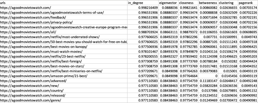
Skewed Distribution of Small Numbers

Now that we have our centrality metrics, we can begin our analysis and interpretation. I’ll explore auditing and analysis in a future post, but for now, I want to discuss some transformations we can apply to our data. This process is helpful because centrality metrics can be a bit unwieldy on large graphs.

When you look at your centrality metrics, you’ll find two things. First, the numbers are very, very small. Second, the distribution is intensely skewed and heavy-tailed. Let’s look at a basic solution for the first problem, then let’s look at a combination of PageRank issues.

Scaling Our Metrics

A simple method for scaling our centrality metrics is to set our max value to 1 and scale down all other scores as a percentage of that max score. These relative metrics may be a bit easier to interpret. Here is an example with the output limited to the first 5 rows.

max_value = max(betweeness_centrality.items(), key=lambda x: x[1])

bc_scaled = {}
for k in betweeness_centrality.keys():
    bc_scaled[k] = betweeness_centrality[k] / max_value[1]

sorted(bc_scaled.items(), key=lambda x:x[1], reverse=True)[0:5]

Output:

[(‘https://agoodmovietowatch.com/advanced/’, 1.0),
(‘https://agoodmovietowatch.com/new/’, 0.34161086672951907),
(‘https://agoodmovietowatch.com/lists/staff-list/’, 0.23675308508646625),
(‘https://agoodmovietowatch.com/country/’, 0.12338744852904392),
(‘https://agoodmovietowatch.com/the-very-best/’, 0.11990747797772154)]

These numbers are larger and measured relative to the URL with the max Betweenness Centrality.

Now let’s look at PageRank in more depth and try to solve both the scale and distribution challenges we’ll face.

What Does a PageRank Score Mean?

In the last post, I talked about the calculation of PageRank, but what does a PageRank value of “8.002E-07” even mean?

First, if you’re not familiar with the scientific notion (the E-07), that means we move the decimal to the left by 7 positions. That makes the PageRank value “0.0000008002.” That number is the probability of a random non-biased user being on that page at any given moment in an infinite random crawl (tweaked this definition thanks to feedback from @willcritchlow).

Since PageRank is the probability of being on one of your pages, adding all your PageRank scores together will equal 1. We can even add these up by groupings of pages (page type, site section, topical).

We’re unlikely to find a uniform or normal distribution of probabilities. The distribution of PageRank is typically highly skewed with a heavy tail. Some common SEO strategies are actually designed to affect the distribution of PageRank by pushing it towards a flatter or more normalized distribution.

These skewed distributions of very small numbers can be cumbersome to interpret. We’ll look at that problem in just a moment, but first, let’s talk about the zero-sum nature of PageRank.

Internal PageRank is a Zero-Sum Game

Because PageRank adds up to a whole of 1, think of PageRank as dividing up a pie. It’s a finite resource that is distributed across all your pages. You cannot increase the internal PageRank of a page without taking it from somewhere else. There are opportunity cost trade-offs associated with influencing your PageRank distribution.

This also means that the more “higher” PageRank pages you have, the lower your highest PageRank score may be.

Most sites have a PageRank inequality issue where a small number of URLs have a high PageRank, and 85%+ of the URLs have very small PageRank. We often want to close the PageRank gap a bit, but we can only go so far. We also don’t want a uniform distribution where no page is more valuable than any other. There will always be “losers” when we try to prioritize certain pages.

External links make the pie bigger, but PageRank still represents what percentage of the pie a URL gets based on the internal link structure. We aren’t factoring external links into our calculation, but I’ll look at that in my next post.

Let’s look at our demo site’s distribution and see if we can make it easier to understand.

Understanding Our PageRank Distribution

We can do a few things to get an idea of the characteristics of our PageRank distribution.

A) Calculate Kurtosis and Skewness

We can run some basic descriptive statistics to understand our distribution without plotting it. For this, we’ll use the SciPy package.

print("Kurtosis: %s" % stats.kurtosis(df_metrics['pagerank']))
print("Skewness: %s" % stats.skew(df_metrics['pagerank']))

Output:

Kurtosis: 67.81416670009466
Skewness: 8.212411833211922

Kurtosis is a measurement of the tailedness of a distribution. It lets us know if the tail of our distribution contains extreme values. The kurtosis of a normal distribution is 3, so the excess kurtosis is 53.39-3 = 50.30. This lets us know we have a heavy tail.

Skewness is a measure of the asymmetry of the probability distribution. Our distribution is highly skewed. A positive skew means the right tail is longer, and the bulk of the probability is concentrated to the left.

B) Plot Histogram

Next, we can plot our PageRank scores as a histogram to visualize their distribution. This should confirm what we already know from our descriptive statistics.

pr_list = list(df_metrics['pagerank'])
n, bins, patches = plt.hist(pr_list, 10, facecolor='g', alpha=0.75)

plt.xlabel('PageRank')
plt.ylabel('Count')
plt.title('PageRank Distribution')
plt.xlim(0, 0.01)
plt.grid(True)
plt.show()

Output:

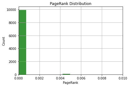
This visualization isn’t helpful. The overwhelming majority of nodes have a very low PageRank, and just a few have relatively higher PageRank.

We can make it a bit better by plotting this with a log scale on the Y-axis. We do this by adding the following to the code above.

plt.yscale('log')

Output:

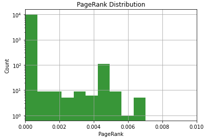
This is a bit better, but be careful with that Y-axis. Don’t forget it’s a log scale on the Y-axis. There are a lot more URLs in that first bin than the second one.

Lastly, we could also plot a QQ plot, which compares two probability distributions. We could use it to see how much the distribution differs from a normal distribution.

Log Transformation to a 10 Point Scale

A log transformation of a skewed distribution can help normalize it. By log transformation, I simply mean taking the log base 10 of our PageRank values. A log transformation makes highly skewed data less skewed, which can make our data easier to interpret. This can also give us a 10 point log scale PageRank similar to the old school “Toolbar PageRank.”

The calculation is simple:

log10(pagerank)

However, all of our values are less than one, so the log will return a negative number. We can fix that by shifting the curve up by adding to the outcome of the log10(pagerank) result. We simply add a constant C.

log10(pagerank) + C

One question to consider is what number we should use to shift the curve? How do we anchor it to a 10 point scale? What should the “C” be in the equation above? There are a few choices that I’ve observed in various SEO tools.

• Anchor Max PageRank as 10: This will give the highest page on a site a PageRank of 10, and scores will scale down from there. A PageRank score of 9 will have ten times less PageRank than the highest PageRank on the site. We calculate this constant (“C”) by determining the absolute value of the difference between the max log10(pagerank) and 10. We add that constant to the log(pagerank) outcome.
• Anchor Min PageRank to 0 or 1: This will give the lowest page a zero or one score. It’s the same concept as anchoring at 10, except now your reference point is the minimum.

Both of these have some issues that I don’t like:

• Relative Anchoring is Misleading: It can misleading to say a URL has a PageRank of 10. Where does it go from there? It can make you think a URL is “doing well” when all the 10 means is that the URL has the highest PageRank in a single crawl. If you anchor to the bottom, you end up with many low scores, which is equally misleading.
• Relative to a Given Crawl: If the constant is based on the max or minimum, it changes crawl to crawl. This makes comparisons overtime useless. An 8 today isn’t the same as an 8 two months ago. An 8 means a URL’s PageRank is 100 times less than the maximum for that crawl (if we anchored max at 10), it doesn’t mean it has a specific amount of link value or PageRank from crawl to crawl.

Instead, let’s use shift the curve by a constant that’s independent of a crawl. I like to use 10 for a few reasons.

• It’s a nice even number. 10 is a good number.
• The maximum PageRank possible is 1. The log of 1 is 0. The maximum possible PageRank will be anchored to 10.
• For the log transformation to be less than -10 (and therefore our 10-point score would be less than zero), the PageRank would have to be smaller than 1E-10, which is 1 divided by 10 billion. Many sites don’t have enough nodes to get PageRank scores that small. This means a zero on our scale has a worse than a 1E-10 probability of being discovered.
• A constant shift means an 8 today equals an 8 a few months ago. They both represent the same raw PageRank value. (Although PageRank itself is a bit of a relative value.)

A constant of “10” might not work for huge sites. If the raw PageRank gets low enough, you will get back a negative number (unless you clip at zero). In that case, you could anchor the max value approach or come up with a different constant that works for your site. Most sites don’t change size radically, so you could stick with whatever number you choose for a while.

Our formula will be:

log10(pagerank) + 10

To prevent any edge case from falling below 0, we can clip our calculated values at 0 and 10. If log10(pagerank) + 10 is less than zero, it gets zero. This can occur if a URL’s raw PageRank is less than 1E-10.

Once we’ve transformed PageRank, they can no longer be summed. Transformed PageRank is simply a type of scaling to help us make sense of the raw PageRank values.

Calculating a 10-point PageRank

This calculation outlined about is fairly straight-forward.

df_metrics['internal_pagerank_score'] = np.clip(np.round(np.log10(df_metrics['pagerank']) +10, decimals=2), 0, 10)

Here is what we’re doing in the code from left to right:

• Storing the output into a new column in our metrics DataFrame
• Clipping the output of our calculation, so it doesn’t go outside the range of 0 to 10.
• Rounding the result of our log transformation to two decimal points.
• Taking the log base 10 of the PageRank value.
• Shifting the curve up by 10

Let’s plot a histogram of our new calculated 10-point PageRank score.

bins = [0.5, 1, 1.5, 2, 2.5, 3, 3.5, 4, 4.5, 5, 5.5, 6, 6.5, 7, 7.5, 8, 8.5, 9, 9.5]
n, bins, patches = plt.hist(list(df_metrics['internal_pagerank_score']), bins, facecolor='g', alpha=0.75)
plt.xlabel('Internal PageRank Score (Log Transformation)')
plt.ylabel('Count (Log Scale)')
plt.title('PageRank Distribution')
plt.xlim(0, 10)
plt.yscale('log')
plt.grid(True)
plt.show()

Output:

PageRank is now in a form that SEOs are more accustomed to evaluating. The distribution is also much easier to understand, but be careful when assessing this chart as both the X and Y axes are log. Each unit increase in PageRank is a 10X change in raw PageRank (probability). I’m also using a log scale for the y-axis. Each line is a 10X increase in count.

We can now export out DataFrame to CSV again to evaluate in Excel.

df_metrics.to_csv('data/large-graphs/centrality-metrics.csv')

We can check the Kurtosis and Skewness again to how it changed.

print("Kurtosis: %s" % stats.kurtosis(df_metrics['internal_pagerank_score']))
print("Skewness: %s" % stats.skew(df_metrics['internal_pagerank_score']))

Output:

Kurtosis: 19.227319660457127
Skewness: 4.111278422179072

Our distribution is still heavily skewed and tailed, but much less than before the log transformation.

Resources for Even Larger Graphs

At the beginning of the post, I mentioned that you might run into the limits of NetworkX. For very large graphs, you’ll want to use a package written in C/C++. Several good ones interface with Python.

The syntax and APIs for these packages are not as intuitive as NetworkX, so you could argue they’re not as beginner-friendly. There is also additional installation effort required (installing a C/C++ compiler). Additionally, the graph storage methodology used by some of these alternatives can make some actions less flexible. Lastly, one of the challenges you’ll face is a disparity in the algorithms and visualization features available across the options. With those caveats out of the way, let’s look at some alternatives to NetworkX.

Tools That Handle Very Large Graphs

• iGraph – iGraph is very similar to NetworkX. It’s a C library but works with Python and R. It is 10 to 50 times faster than NetworkX, which makes it better for networks with greater than 100K nodes. It also has unique features you don’t find in NetworkX. However, it requires a compiler and more effort to install. Some challenges arise based on how iGraph stores its nodes and edges.
• graph-tool – This is also written in C/C++. It is good at taking full advantage of all CPUs/cores and parallel calculations. This can reduce the run time of complex calculations, like PageRank, on very large graphs. It also has several unique features. However, the installation process can be a challenge. 
• NetworKit – This is also written in C/C++ but is compatible with NetworkX at the graph level. This means you can use NetworkX to construct your graph, then transfer it over to NetworKit for more intensive analysis.

There are more options than this, but these are some of the popular ones I’m familiar with.

Relative Speed of Each Package

You’ll find that different algorithms run more efficiently on various packages. You’ll also find that some algorithms take better advantage of multi-threading.

I recommend this post that runs algorithm benchmarks across multiple datasets with five different packages. It does some rigorous testing on a fast machine (16 Cores with 60GB of ram)

They found that NetworkX was 10X slower the second slowest package. They normalized the benchmarks by calculating how many more times you could run an algorithm in the time it took NetworkX to complete it. For some of these algorithms, they’re hundreds of times faster than NetworkX (although different packages use different methodologies in their algos, so it’s not always apples-to-apples).

Why NetworkX If It’s Slow?

It’s easier to install, use, and understand. It’s well documented and has an active community as well. This makes it easy to learn and find help. It can also handle large enough graphs to cover most websites that most SEOs work with.

If you’re new to Python or graph analysis, it’s an excellent place to start. Once you have the language and concepts down, it’s easier to pull in other tools as needed.

Introduction to iGraph

I’m not going to go in-depth on iGraph, but here is a quick overview of how to get our DataFrame into iGraph, calculate PageRank, export it to CSV, and bring it back into a Pandas DataFrame. Its calculation speed is much, much faster than NetworkX. If you’re exceeding 100K nodes, you may need to use iGraph.

Installation

Follow the installation instructions here (skip down to the section for your OS). There are a couple of approaches, and it varies by OS. I’m on Mac, and I had Xcode Command Line Tools installed, so I could install ‘python-igraph’ using pip and didn’t run into any issues. I believe you can install Xcode Command Line Tools with “xcode-select –install” in terminal. (Note that this can get a bit more complicated on Windows. I don’t code on any of my Windows machines, so I’m not much help.)

Preparing Our Data

Creating our graph is easier if we format our DataFrames to work nicely with iGraph. For our edge DataFrame (df) this means having the first two columns as our source and target, followed by any columns we want to use as edge attributes (such as link score as weight). For our node DataFrame (df_nodes), this means setting our node names to the first column and following it with anything we want to be a node attribute.

To do this, I’m going to drop some columns from both of our DataFrames.

df = df.drop(columns=['type','status_code','follow','link_position'])
df_nodes = df_nodes.drop(columns=['node_id'])

Create Graph

Next, let’s create a graph in iGraph using the data from our two DataFrames. It’s worth mentioning that the terminology in iGraph is a bit different, such as nodes being called vertices.

import igraph
G2 = igraph.Graph.DataFrame(df, directed=True, vertices=df_nodes)

I created a graph from a DataFrame, used “df” as the edges, set it to ‘directed,’ and set vertices based on our node list DataFrame. Setting our vertices parameter will pass over the URL labels as names for our vertices (nodes).

Calculate PageRank

Calculating PageRank is easy (and super fast). It took less than a second for our demo site.

g2_pagerank = G2.pagerank()

Exporting PageRank to CSV

Let’s export our list of PageRank scores to a CSV. If you look inside “g2_pagerank,” you’ll see that it’s just a list of scores without the vertices (nodes) associated (no URL information). We need to combine the names of the vertices with their score before we write to CSV.

import csv

with open('data/large-graphs/g2-pagerank.csv', mode='w') as pagerank_export:
    writer = csv.writer(pagerank_export, delimiter=',', quotechar='"', quoting=csv.QUOTE_MINIMAL)
    writer.writerow(['url', 'ig_pagerank'])
    for v in G2.vs:
        writer.writerow([v['name'], g2_pagerank[v.index]])

Most of this is fairly straightforward. I imported “csv” so we can open and write a CSV file. I wrote the first row with the column names. Next I’m looping through each of the vertices (nodes) in G2 (accessed with “.vs”) and for each I’m writing out the name attribute and the corresponding PageRank score from our list of calculated scores (with the same index).

iGraph PageRank to a DataFrame

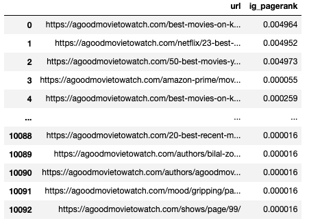
We can use the same process to save it to a DataFrame in Pandas.

df_ig = pd.DataFrame(columns=['url', 'ig_pagerank'])
for idx, node in enumerate(G2.vs):
    df_ig.loc[idx] = [node['name'], g2_pagerank[idx]]
df_ig

Output:

My Thoughts on iGraph

The speed of iGraph is impressive. The install can be more work than NetworkX, but it’s was pretty easy on my Mac. I don’t like the documentation as much as NetworkX, and it’s also harder to find example code or help. Lastly, I don’t find it as intuitive as NetworkX, but it’s still pretty simple. Some things that were easy to do with NetworkX seem to require just a bit more code.

If you’re working with very large graphs, the speed of iGraph could save you minutes, if not hours, of time waiting for your algorithms to calculate.

Memory Limitations of Pandas

Before we wrap up, it’s worth mentioning that you can also run into memory limitations with Pandas. You can help this, to an extent, by increasing the memory on your machine, but you may still run into some limits. Even if your DataFrame uses only a portion of your memory, Pandas can still hit your ceiling due to some functions requiring duplicate copies of your DataFrame to compute.

We’ve covered some of the tools to reduce memory usage in this post, such as limiting your columns and changing data types to something more memory efficient. If that isn’t enough, there are two other options available.

• Chunking: Chunking allows you to read in chunks of your data at a time (loop through CSV by reading N number of rows at a time). You can then perform your required work on that subset and then save it out to a DataFrame.
• Use Dask: Dask is a parallel computing library and has a DataFrame API. It can use multiple threads or use a cluster of machines to process data in parallel. I haven’t needed to use this yet, but I wanted to mention it.

What’s Next?

Hopefully, this post made ingesting and analyzing larger graphs a little more manageable. In my next post in this series, I’ll look at customized/personalized PageRank, communities, strongly connected components, subgraphs, and visualizations. After that post, I’ll get into auditing, analysis, and actionable insights derived from this data.